
Introduction
ChatGPT has rightly taken the world by storm, and has possibly started the 6th wave. Given its importance, the rush to build new products and research on top is understandable. But, I’ve always liked to ground myself with foundational knowledge on how things work, before exploring anything additive. To gain such foundational knowledge, I believe understanding the progression of techniques and models is crucial to comprehend how these LLM models work under the hood.
Inspired by Andrej Karpathy’s enlightening ‘makemore’ series, this post aims to dive deep into the key academic papers that shaped our current landscape of language models. From Recurrent Neural Networks (RNNs) to Transformers, let’s demystify these complex concepts together.
As of the time of this writing, Andrej hasn’t updated his series in the last 6 months. This leaves a gap in our comprehension as the series jumps from WaveNets to Transformers and GPT. Hence, I’d like this blog to act as a bridge, filling the void for anyone on a similar journey of understanding. Rest assured, when Andrej completes his series, it will serve as a comprehensive resource. Meanwhile, let me summarise as best as I can.
Papers NOT be going through
The following papers are ones, that andrew has explained in a lot of detail in his make more lecture series on YouTube , and I would recommend anyone to go through the series - as its the best explanation I’ve seen so far.
Bigram (one character predicts the next one with a lookup table of counts)
MLP, following Bengio
CNN, following DeepMind WaveNet 2016
Papers intend to deep-dive into:
RNN , following Mikolov et al. 2010 Recurrent neural network based language model
Bidirectional RNN, following Mike et al 1997 paper
Backpropagation through time , followed in Mikael Bod ́en 2001 BPTT
LSTM , following Graves et al. 2014 Generating Sequences With Recurrent Neural Networks
GRU , following Kyunghyun Cho et al. 2014 On the Properties of Neural Machine Translation: Encoder–Decoder
Batch Normalisation, following Sergey Ioffe et al. 2015 Batch Normalization: Accelerating Deep Network Training by Reducing Internal Covariate Shift
Layer Normalization, following Jimmy Lei Ba, 2016 Layer Normalization
Attention, following Dzmitry Bahdanau, 2015 Dzmitry Bahdanau, 2015
Transformers , following Vaswani et al. 2017 Attention Is All You Need
Let’s get started
RNN - Recurrent Neural Networks
Paper: Mikolov et al. 2010
Summary
The primary challenge that this paper addresses is sequence prediction: given X tokens of a sequence, predict the X+1th token. While the bigram and MLP papers solved this by feeding some fixed context-length to predict the next token, they had their shortcomings - namely fixed and manually set context lengths. To overcome these, the authors propose how a recurrent neural network can “figure-out” the context length instead of manually setting it.
The proposed RNNs, can “build a context” of information from the past and incorporate it into their predictions. This feature allows RNNs to capture dependencies between elements in a sequence, making them especially suited for tasks involving sequential data.
The problem, in the words of the author:-
It is well known that humans can exploit longer context with great success. Also, cache models provide comple-
mentary information to neural network models, so it is natural to think about a model that would encode temporal information
implicitly for contexts with arbitrary lengths
The solution
The authors then explain how a simple recurrent neural network works
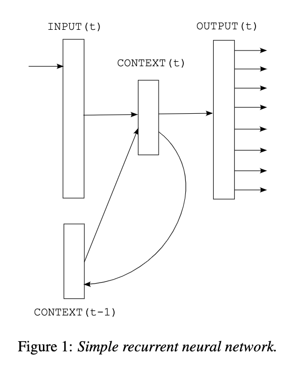
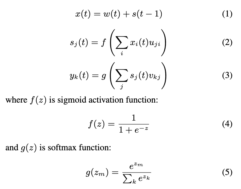
Where
w(t) is the input word at t
s(t-1) is the state previously generated by the RNN in its last time-step
Output layer y(t) represents probability distribution of next word given previous word w(t) and context. Consequently, time needed to train optimal network increases faster than just linearly with increased amount of training data: vocabulary growth increases the input and output layer sizes, and also the optimal hidden layer size increases with more training data.
Back-propagation through time (BPTT) algorithm is used. (This is covered next)
How do you back-propagate through the loop ?
Backpropagation through time , followed in Mikael Bod ́en 2001 BPTT
The key insight is around how to back-propagate through the recursion caused loop
The solution is to “unroll” the model T times, and then follow normal backpropation
Instead, of keeping separate weight matrix for each time-step, the weight matrix is instead shared across the unfolded layers.
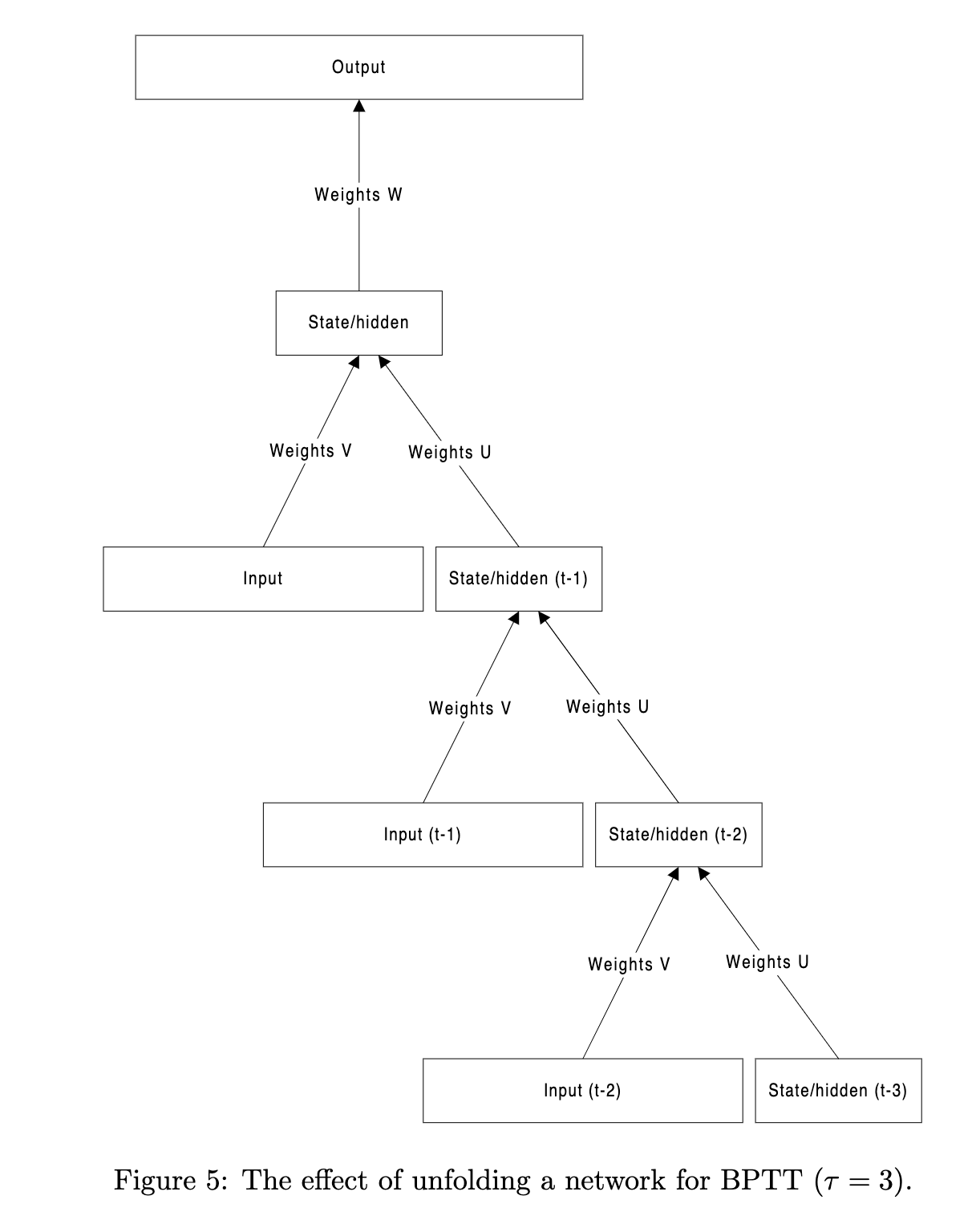
Note, how weights V and U , remain the same through the unfolding process
Important quotes from the paper:
It is important to note, however, that after error deltas have been calculated, weights are folded back adding up to one big change for each weight. Obviously there is a greater memory requirement (both past errors and activations need to be stored away), the larger τ we choose.
In practice, a large τ is quite useless due to a “vanishing gradient effect” (see e.g.
(Bengio et al., 1994)). For each layer the error is backpropagated through the error
gets smaller and smaller until it diminishes completely. Some have also pointed out that the instability caused by possibly ambiguous deltas (e.g. (Pollack, 1991)) may disrupt convergence. An opposing result has been put forward for certain learning tasks (Bod ́en et al., 1999).
Note: Batch normalization and layer normalization were probably not present at this time.
Notable lines from the paper:-
Based on our experiments, size of hidden layer should reflect amount of training data - for large amounts of data, large hidden layer is needed
Convergence is usually achieved after 10-20 epochs.
regularization of networks to penalize large weights did not provide any significant improvements.
PyTorch
Input:
(N,L,H**in) when batch_first=True
N = Batch Size
L = Sequence Length
H_in = Hidden Layer
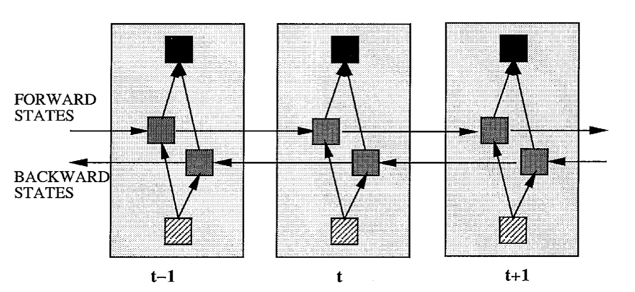
Bidirectional RNN
Paper: Mike et al 1997 paper
Future input information coming up later than is usually also useful for prediction. With an RNN, this can be partially
achieved by delaying the output by a certain number of time frames to include future information. While delaying the output by some frames has been used successfully to improve results in a practical speech recogni-
tion system [12], which was also confirmed by the experiments conducted here, the optimal delay is task dependent and has to be found by the “trial and error” error method on a validation test set.
To overcome the limitations of a regular RNN outlined in the previous section, we propose a bidirectional recurrent
neural network (BRNN) that can be trained using all available input information in the past and future of a specific time frame.
LSTM - Long Short-term Memory
Paper: Graves et al. 2014 Generating Sequences With Recurrent Neural Networks
Summary
Quoting the paper to best describe the problem they are addressing
In practice however, standard RNNs are unable to
store information about past inputs for very long [15]. As well as diminishing
their ability to model long-range structure, this ‘amnesia’ makes them prone to
instability when generating sequences. The problem (common to all conditional
generative models) is that if the network’s predictions are only based on the last
few inputs, and these inputs were themselves predicted by the network, it has
little opportunity to recover from past mistakes. Having a longer memory has
a stabilising effect, because even if the network cannot make sense of its recent
history, it can look further back in the past to formulate its predictions.
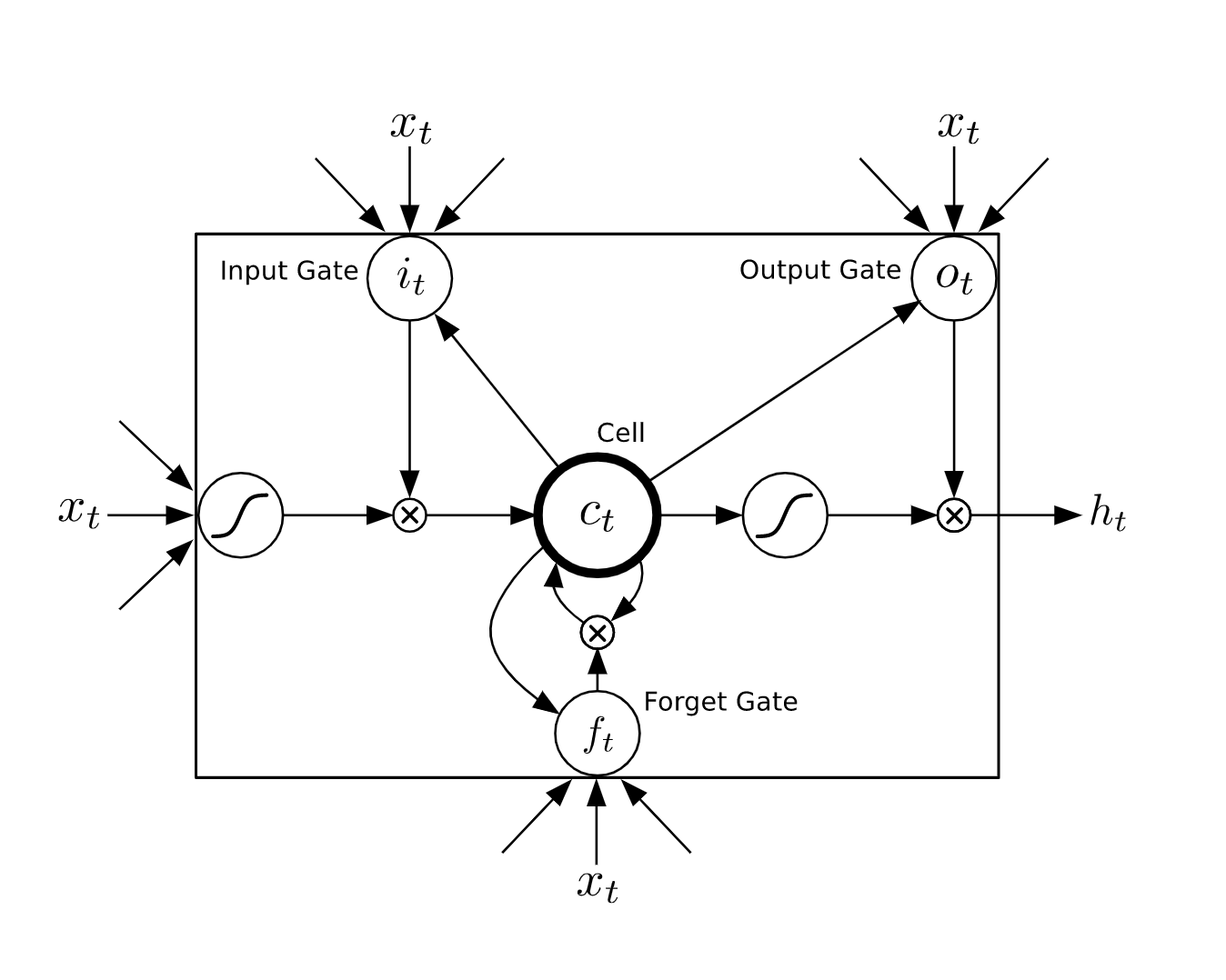
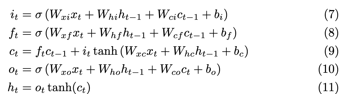
In my words, I understand it as follows
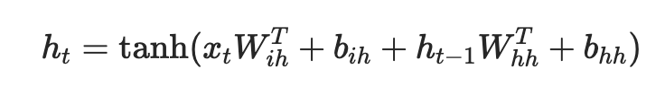
The forget gate, tries to find how much to forget in the next iteration. The network learns weights, such that for certain inputs x, at hidden states h and a previous cell state c[t-1] - it predicts how to forget in the next iteration
Simlarly, the input gate learns how much to store in the new cell state at t.
Combining both, the new c[t] is a Fc[t-1] + I(WX+Wh+b)
The paper has some great examples of text generation and handwriting prediction using LSTMs, that I would encourage going through.
Paper 2 by Google: hasim et al. 2014 hasim et all
The recurrent connections in the
LSTM layer are directly from the cell output units to the cell input
units, input gates, output gates and forget gates. The cell output units
are connected to the output layer of the network.
PyTorch:
Reference: https://pytorch.org/docs/stable/generated/torch.nn.LSTM.html
GRU - Gated Recurrent Neural Networks
Paper:
Cho et. al 2014 Learning Phrase representations using Encoder-Decoder
On the Properties of Neural Machine Translation: On the Properties of Neural Machine Translation: Encoder–Decoder
paperFrom the Papers:
In addition to a novel model architecture, we also
propose a new type of hidden unit (f in Eq. (1))
that has been motivated by the LSTM unit but is
much simpler to compute and implement.1 Fig. 2
shows the graphical depiction of the proposed hidden unit.
We show that the neural machine translation performs
relatively well on short sentences without unknown words,
but its performance de-grades rapidly as the length of the sentence
and the number of unknown words increase.
Furthermore, we find that the pro-posed gated recursive convolutional net-
work learns a grammatical structure of a sentence automatically.
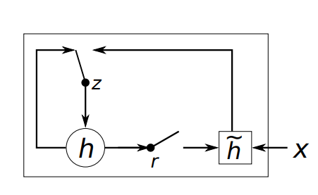
In my words, they simplified the task to an update gate and a reset gate, instead of the complicated interactions between multiple gates in LSTMs.
Both the reset gates and update gates are a function of the input, and the hidden state at t-1
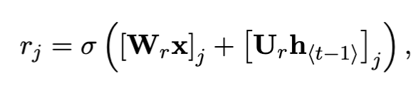
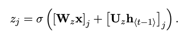
and the next h state is calculated as
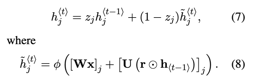
As each hidden unit has separate reset and update gates, each hidden unit will learn to capture
dependencies over different time scales.
Those units that learn to capture short-term dependencies
will tend to have reset gates that are frequently active, but those that capture longer-term dependencies will have update gates that are mostly active.
Batch Normalisation
Paper: [[Batch Normalisation]], following Sergey Ioffe et al. 2015 Batch Normalization: Accelerating Deep Network Training by Reducing Internal Covariate Shift
The problem
Training is complicated by the fact that the inputs to each layer
are affected by the parameters of all preceding layers – so
that small changes to the network parameters amplify as
the network becomes deeper.
Change in the distributions of layers’ inputs presents a problem because the layers need to continu-
ously adapt to the new distribution.
Input distribution properties that make training more efficient – such as having the same distribution
between the training and test data – apply to training the sub-network as well. As such it is advantageous for the
distribution of x to remain fixed over time.
Consider a layer with a sigmoid activation function z = g(W u + b) where u is the layer input,
the weight matrix W and bias vector b are the layer parameters to be learned, and g(x) = 1/ 1+exp(−x) . As |x|
increases, g′(x) tends to zero. This means that for all dimensions of x = W u+b except those with small absolute values, the gradient flowing down to u will vanish and the model will train slowly.
If, however, we could ensure that the distribution of nonlinearity inputs remains more
stable as the network trains, then the optimizer would be less likely to get stuck in the saturated regime,and the training would accelerate.
So they propose a new solution
The Solution:
Introduce a normalization step that fixes the means and variances of every layer inputs
What they tried: One approach could be to modify the network directly at regular intervals, to maintain the normalisation properties. They explain that this doesn’t work because
The issue with the above approach is that the gradient descent optimization does not take into account the fact that the normalization takes place.
We have observed this empirically in initial experiments, where the
model blows up when the normalization parameters are
computed outside the gradient descent step
And hence they proposed the solution to bring the batch-normalisation layer
To address this issue, we would like to ensure that, for any parameter values,
the network always produces activations with the desired
distribution. Doing so would allow the gradient of the
loss with respect to the model parameters to account for
the normalization, and for its dependence on the model
parameters Θ
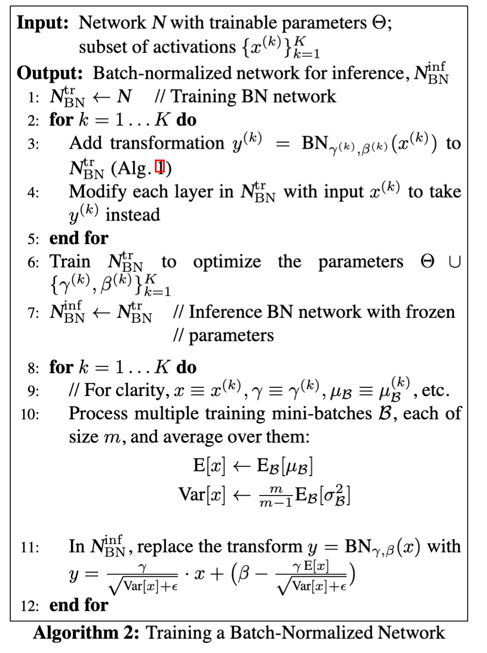
The Batch Normalisation Layer Algo
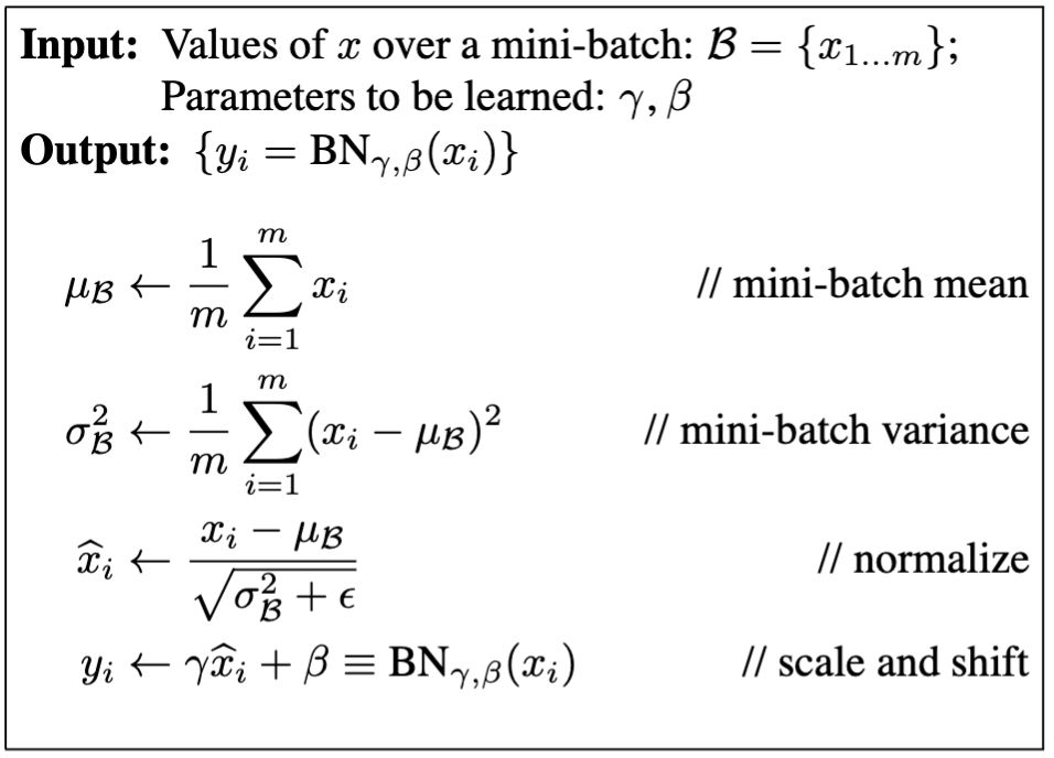
Important points:
Normalises dimensions independently:
The algorithm works to normalise each dimension independently. So for each dimension k, it hopes to normalise
Enables the layers to still adapt
It’s important to not change what each layer represents. So they don’t want to specifically force every activation to be of mean 0 and variance 1. Instead, they introduce the scaling parameters to let the network still learn the biases and scaling factors. The algorithm merely ensures that the distribution of the inputs is maintained.
This is done via
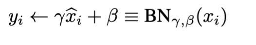
Note that this enables the network to retain the representation
Cons: Creates coupling between the examples in the training
Rather, BNγ,β (x) depends both on the training example and the other examples in the mini-batch.
The BN layer is differentiable:
Normalization is only needed during training
The normalization of activations that
depends on the mini-batch allows efficient training, but is
neither necessary nor desirable during inference
Hence after training, only the population statistics is used for the providing the same effect during inference
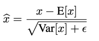
These statistics are calculated by using moving average method
We use the unbiased variance estimate Var[x] = m
m−1 · EB[σ^2 ], where
the expectation is over training mini-batches of size m and σ^2 are their sample variances
Since the means and variances are fixed during inference,
the normalization is simply a linear transform applied to
each activation.
Final Algorithm
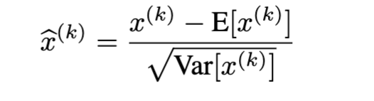
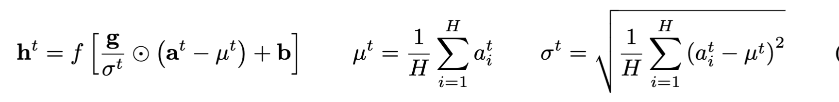
Layer Normalisation
Paper: [[Layer Normalization]], following Jimmy Lei Ba, 2016 Layer Normalization
The problem
Batch normalisation depends on mini-batches, and it isn’t obvious how to use them in an RNN model
In feed-forward networks with fixed depth, it is straightforward to store the statistics separately for each hidden layer. However, the summed inputs to the recurrent neurons in a recurrent neural network (RNN) often vary with the length of the sequence so applying batch normalization to RNNs appears to require different statistics for different time-steps.
The change is to calculate the mean and variance statistics over all the hidden units in a layer, instead of the batches
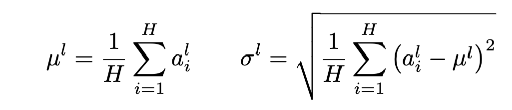
After that, the famliar bias and gain are added, similar to BN
Attention: Neural Machine Translation
Paper: Attention, following Dzmitry Bahdanau, 2015 Dzmitry Bahdanau, 2015
Background
This paper was trying to solve language translation problems, and while the title doesn’t focus on attention - this is the first time that the mechanism of “attention” was provided. So it brings us to the foundations of how attention came to be.
At the time of this paper, the encoder-decoder architecture is prominent for translation. Namely, a bidirectional RNN is used to encode the source sentence, and the decoder RNN is conditioned on the output of this encoder RNN to produce the translated sentence.
Problem
In the words of the author:
A potential issue with this encoder–decoder approach is that a neural network needs to be able to compress all the necessary information of a source sentence into a fixed-length vector. This may make it difficult for the neural network to cope with long sentences
Solution Abstract:
Introduce an extension to the encoder–decoder model which learns to align and translate jointly. Each time the proposed model generates a word in a translation, it (soft-)searches for a set of positions in a source sentence where the most relevant information is concentrated. The model then predicts a target word based on the context vectors associated with these source positions and all the previous generated target words.
Architecture
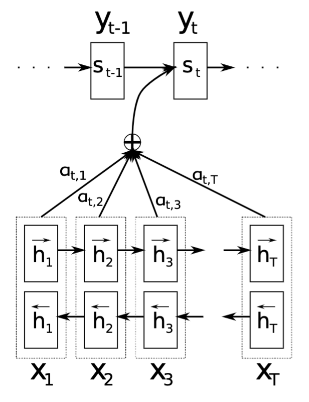
The authors propose a novel architecture, each output word in the decoder is created by considering not only the previous hidden state of the decoder, but also considering a context vector C of the encoder network outputs. This context vector itself is a weighted sum of the hidden states of the encoder network, where the weights are trained and learn the “alignment” between output words and input words.
Math
i, is used for the decoder network , and the j is used for the encoder networks
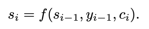
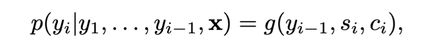
The hidden states s[i] of the decoder RNN are calculated as a function of s[i-1], y[i-1] and c[i]
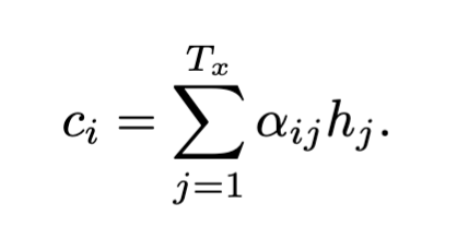
The context vector c[i] is calculated as a weighted sum of all the encoder hidden states h[j]
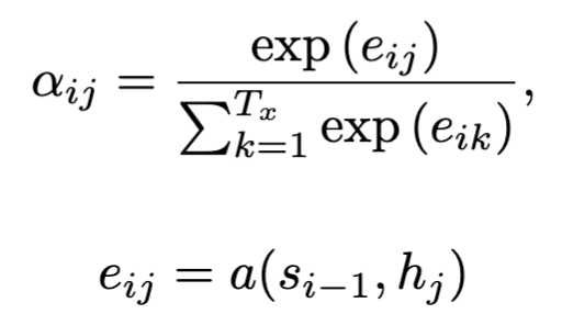
These α weights are an important piece here. These represent the “alignment” of the decoded word to the encoded sentence. Hence, these are trained to be a function of s[i-1], and h[j]. Essentially, the weights help the model understand how much of the j_th input word is resposible for translating the ith output/decoded state.
Note:
We parametrize the alignment model a as a feedforward neural network which is jointly trained with all the other components of the proposed system. the alignment model directly computes a soft alignment, which allows the gradient of the cost function to be backpropagated through.
Finally, p(y) is conditioned on previous words, hidden state s[i], and the context vector c[i]
The Golden Words
The probability αij , or its associated energy eij , reflects the importance of the annotation hj with respect to the previous hidden state si−1 in deciding the next state si and generating yi. Intuitively, this implements a mechanism of attention in the decoder. The decoder decides parts of the source sentence to pay attention to.
By letting the decoder have an attention mechanism, we relieve the encoder from the burden of having to encode all information in the source sentence into a fixedlength vector. With this new approach the information can be spread throughout the sequence of annotations, which can be selectively retrieved by the decoder accordingly.
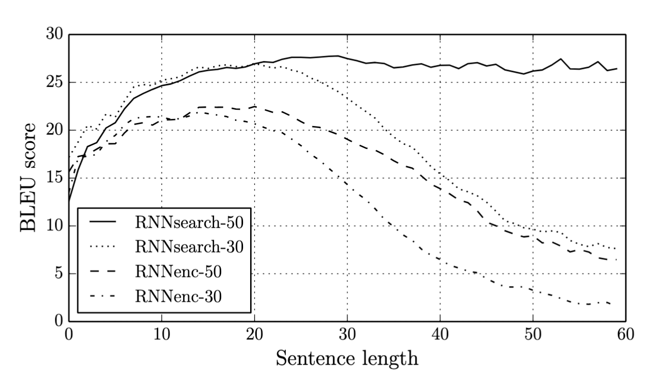
Results
In the next post
Now thats we’ve covered some of the basics from RNNs to Attention, we’ll cover more advanced topics in the next post.
Conclusion
A detailed analysis of each influential paper in this domain can facilitate a comprehensive understanding of these models. Recognizing the limitations of each model and how succeeding models strive to address them is integral to this exploration.
While the completion of Andrej Karpathy’s series is anticipated, further exploration of these foundational works will serve to strengthen our understanding of modern language models. Anticipate future posts in this series, which will delve into the realm of Transformers.
I invite readers to share their insights on these concepts. Which paper do you consider most intriguing?
If i’ve made errors or haven’t described something correctly - please do comment, help me learn and correct the article for future readers.